MODEL ASPECTS
Aspects of mathematical simulation models
This chapter discusses the following issues:
- What are design variables in models?
- What is a model, a system and the 'real existing world'?
- Which ways of representation and/or notation have mathematical models?
- What is a variable, a state variable, a starting value, a constant and a parameter?
- What are endogenous and exogenous variables?
- What is a block scheme, an analogue scheme and an conceptual model?
This chapter will deal with three kinds of aspects (design variables) of mathematical models that are crucial for designing and developing computer simulation programs, viz.: definitions, representations and numerical problems.
This book is not specifically aimed at mathematical modelling and nor at modelling in a certain field, but some basic knowledge concerning the classification, handling and manipulation of models is necessary in order to be able to handle design systems, like implementing models in MacTHESIS. Without these aspects from the 'modelling world' one can not make any progress in computer simulation. A simulation specialist can not design a detailed and specific model without a team to support him.
1. Definitions
A great number of definitions circulate in the 'world of modelling and simulation'. Someone who considers his or here daily job the production of a mathematical model is only an expert in one speciality, and has a different view from someone who has to produce educational computer simulation programs for secondary and vocational education. The first is occupied with modelling in a specific field of knowledge, the second with simulation and programming. So he or she has to be able to move in many fields (of learning).
Area of definition
The world around us consists of small and large, intricate and simple, comprehended and uncomprehended systems. During its entire existence humanity has tried to classify and describe nature and its systems. Metaphysical systems are supposed to belong to the systems that have not been researched scientifically. So we restrict ourselves to the actually existing (materialistic) systems. Furthermore we restrict ourselves to systems which change in time, i.e. dynamic systems that are a function of time. Non-dynamic systems, defined as static systems, are not writen in the scope of this book.
System versus model
When a designer is told to use a certain real life system for a didactic situation, then such a real life system has to be simulated. This can only be done with a mathematical system and a computer simulation program that can handle (compute) such a model and can visualize (represent) data. A model of the system has to be found. There are hardly any ready made models, so a simulation specialist has to make do with whatever is available. Simulations are therefore mostly only made when an interesting model is available for education. In regular education it is unfortunately very rare that a staff member of a simulation project can develop a model himself or have one developed. In training courses in business concerns it is quite different. They have more facilities and money to add a model maker to a team of developers.
First some definitions will be given regarding a system, an element, the state (of elements) and the matching relations of elements.
System: An arbitrary chosen set of elements that have mutual relations. We can distinguish:
- Dynamic systems, i.e. the system is a function in time.
- Static systems, i.e. the system is not a function in time.
Element: Smallest part of a system. We can distinguish:
- inanimate elements
- living elements (can change the state of the system)
Relation: Describes the connection between elements.
State: Is an inventory of
- the content of the system
- the structure of the system
- the values of the elements (at a certain point of time).
Models
A model can also be called a system, with a number of essential characteristics. An important division used in modelling is whether a model can be noted symbolically or not. According to Boerma and Hoederkamp (1981) there are three kinds of models: analogue models, symbolic models (algebraic, mathematical, Boolean, in target language etc.) and ionic models (when a model cannot be noted symbolically).
Analogue models
Analogue models, i.e. models with 'similar' characteristics. Also called an analogy (analogon), that is a model of a system with the help of another system. Mostly such a model is meant to simulate in a clearly visual way the dynamic behaviour of a system. For example a mass-spring system that is represented by a resistance/condenser network (or reserved). It can concern static as well as dynamic models.
Symbolic models
These models can be described with symbols, so generally in a algebraic of mathematical way. Geometric models are not described in this book. Within the symbolic models a distinction can be made between static or dynamic mathematical models and deterministic or stochastic mathematical models:
(static) algebraic models (for example spreadsheet models):
x = f(x, y, ...)
y = g(x, y, ...)
(dynamic) algebraic models (mostly an analytical solution of a dynamic model):
x = f(t, x, y, ...)
y = g(t, x, y, ...)
(deterministic) dynamic mathematical models:
dx/dt = f(x, y, ... )
dy/dt = g(x, y, ... )
stochastic (dynamic) mathematical mathematical models with at least one stochastic variable in time (for example queuing problems):
dx/dt = f(x, y, ...) + e(t)
dy/dt = g(x, y, ...) + ...
geometric models in the xyz-space:
x1 = ...; y1 = ... ; z1 = ...;
x2 = ...; y2 = ... ; z2 = ...;
x3 = ...; y3 = ... ; z3 = ...;
Iconic models
Mostly an iconic model is strongly visualized and sometimes two dimensional. For example a picture, an architectural plan or a scale model of a building. These are generally static models.
These deterministic and stochastic (dynamic) models naturally always contain at least one differential equation. That is why we will further explain a division of differential equations.
Spatial models (geometric models) which are recorded mathematically in one way or other, for example by three dimensional sets of coordinates, will not be discussed here.
Division in solving methods
Models can also be divided according to the method of solution. Variables in mathematical models can be calculated simply by filling in the value of time in the equation (i.e. when there is an analytical solution), or calculated by numerical methods of solving (when there is no analytical solution).
This division is as follows:
Type 1: when an analytical solution of a mathematical model is known or can be deduced algebraically. By an analytical solution is meant that the mathematical model with differential equations is brought down to one normal equation, in which the value of the variable y can be calculated at any moment t by substituting the value of the time t in the equation(s). The model can then be solved without the numerical approach.
For example the equation y =A.sin(w.t) +B is the analytical solution of a system of two first order differential equations. Most systems of differential equations have no analytical solution and can therefore only be solved with analogue or digital computers.
Type 2: when a solution is possible with the help of an analogue computer. Mathematical models (with differential equations) can yet be solved without having an analytical solution. Formerly this was mostly done with 'analogue computers'. From this period dates the very practical term 'analogue notation' or the more confusing term 'analogue scheme'. (Not to be confused with the term 'analogue model' as described above). Nowadays a numerical solving method is practically always recommended on a digital computer.
Type 3: when a solution with the help of the numerical solving method is necessary, so when there is no analytical solution. This is almost always the case with dynamic models. Dynamic models are described by a system of differential equations. An ordinary digital computer has to be used then. The values of the variables can not be calculated (as in type 1: analytical), but have to be calculated in an interactive process. This book is restricted to deterministic dynamic models, which are described by differential comparisons (or integral comparisons), which have to be solved with numerical solving methods (the method of Euler) and in which the results can be represented numerically or graphically. Stochastic models, in which there are two or more variables, are not included here.
2. Forms of representation of models
Each model of a system can be noted or represented in several ways. Each way of representation or way of notation has its pros and cons, e.g.:
- as a figure, picture or scheme etc. (visual way of notation) (form 1; conceptual model')
- as a text (textual way of notation) (form 2; 'conceptual model')
- as a block scheme (form 3; 'conceptual model')
- as a system of differential equations (form 4)
- as a system of integral equations (form 5)
- as an analogue scheme (analogue notation) (form 6)
- as statements in a computer language (form 7)
Each form of representation can be a 'conceptual model' for another form of representation. The development of a model to be used in a computer simulation program is a step by step process. It always starts with a visual representation of a textual description of the idea (the concept) of how something can be noted down in a different way from what it looks like in reality. Instead of the words conceptual model the term mental model is sometimes used. A famous example of a conceptual model is the first idea of the space shuttle which was sketched on a coaster in a bar.
Below the most important forms will be discussed in detail.
The importance of all these forms of representation of mathematical models lies in the fact that the models (however noted) can be recognized in a scientific magazine or book. They can be transformed eventually into a manageable, numerically solvable model. The model, in fact, has to be a 100% complete. All starting values, parameter values, units, names of quantities etc. have to be collected and processed.
Figure, picture, drawing or scheme (form 1)
Every system can always be described and recorded by a first draft or a drawing. Systems which are coded in such an essentially simple way are also models of the reality of the system which they describe. Visual models of systems are at the same time also conceptual models. For visual models like a draft, a drawing, a figure or a representation, are not a final point in the development of a (dynamic) model. A visual representation is a model of how a system is believed to function (see figure 1).

Figure 1. Conceptual representation of a mathematical model ('conceptual model'). The possibilities for intervention in the model are black (hot spots; inclick regions); the output variables are white circles. (Visualisation of the model).
Text (form 2)
Each system can of course also be described and represented verbally. Textual descriptions of systems are also concepts. In the first phase of a designing process each model exists either as a draft or as a text.
An object lies y(0) meters high. Someone lets the object go.
Due to parameter a the object is pulled to the earth (y=0).
The object falls faster and faster with the speed x. There is
viscous friction (parameter b), etc.
Block scheme (form 3)
After a visual or a textual sketch of a model comes the phase of the inventory of variables, parameters, constants, units and elements of the model. The most schematic form of representation is to note the model in block scheme. This is in fact a 'black box', in which only the input and output variables are indicated. We define the following kind of variables:
- independent (exogenous) (e.g. the input variables p and q)
- dependent (endogenous) (e.g. the output variables x, y and z)
The interventions in a mathematical model can be done by:
- the (model) parameters and/or the (model) constants (e.g. a, b and c)
- the starting values of the state and/or output variables (e.g. y(0), y(0) and z(0) )
- the input variables (e.g. p(t) and q(t) )
The relation between the elements and variables are omitted on purpose. This way of representation of a model plays an important role in getting a complete survey of all aspects which play a role in the model.
The block scheme usually has the output on the right, the input on the left, above and below the constants and/or starting values. Sometimes parameters or constants (as intervention possibilities in the model) are also noted on the left. Constants, parameters and to a certain extent also input variables can be used as possibilities for intervention.
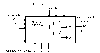
Figure 2. Block scheme or black box model; variables (a), starting values (b), parameters and constants (c):
a: independent (exogenous) versus dependent (endogenous) variables:
p(t), q(t): input variables (exogenous variables);
x(t), y(t): output variable (endogenous variables);
b: state variables:
for example x(t) has influence on an endogenous variable y(t).
Therefore y(t) has actually to be written as y(t,x).
c: parameters, constants and starting values:
a,b and c: parameters or model parameters; some parameters are
sometimes constants.
x(0), y(0): the starting value of x(t) and y(t) at t=0
Each model can be represented schematically in such a way that the so-called dependent (or endogenous) variables are noted as 'output' and the so-called independent (or exogenous) variables as 'input' of a block scheme (see figure 2). The variables which only represent the state of an (internal) sub-model and do not have to occur as 'input' or 'output' can be noted in the block scheme itself. These are called state variables. The model parameters can be noted separately, for example at the top, side or bottom of the block scheme. The starting values of the variables, which can really be considered to belong to the model parameters can also be noted separately, for example at the top. This is a practical and at the same time functional division and way of notation which is useful with complex models (for example systems of more than two differential equations).
Note that parameters, starting values of variables, (model)constants can be used for model interventions. They can nevertheless be used by the students to bring about changes and the students appear to do so. Thus these quantities have become partly dependent on time.
System of differential equations (form 4)
A model can of course be represented as a general system of mathematical equations in which each variable and the possible derivations are dependent on the other variables, on themselves, on the model parameters and on time. Thus a model can initially look like:
x = f (x, y, ... z, dx/dt, dy/dt, ... dz/dt, t, a, b, ... c)
y = g (x, y, ... z, dx/dt, dy/dt, ... dz/dt, t, a, b, ... c)
z = h (x, y, ... z, dx/dt, dy/dt, ... dz/dt, t, a, b, ... c)
However, a mathematical model is hardly ever represented like this. This representation form is only mentioned here for the sake of completeness. Dynamic models are, on the other hand, always represented as systems of differential or integral equations.
Each dynamic model can be written in the form of a system of first order differential equations. The 'dx/dt's' (the derivation of x; the so-called deviation) is put on the left and on the right (in the so-called right term) all variables, parameters, including time are put in principle.
dx/dt = f (t, x, y, ...z, a, b, ...c)
dy/dt = g (t, x, y, ...z, a, b, ...c)
dz/dt = h (t, x, y, ...z, a, b, ...c)
It can be seen that the integrand of the following system of integral equations corresponds with the right term of the corresponding differential equation.
The right terms of the system of first order differential equations appear 'unimpaired' as integrand in the model noted in the integral equations form, but also at the input of the integrator in the analogue notation and as statement in Pascal notation.
System of integration equations (form 5)
Each dynamic model can be noted in the form of a system of integral equations. When the model is written in the form of a system of integral equations it is necessary that starting values are given. That is the value of the variable at the point of time t=0. The right term of the equations acquires yet another term then, namely x(0), y(0), ... z(0). So:
x = ∫ f (x, y, ...z, t, a, b, ... c). dt + x(0)
y = ∫ g (x, y, ...z, t, a, b, ... c). dt + y(0)
z = ∫ h (x, y, ...z, t, a, b, ... c). dt + z(0)
with t from t = 0 until t = T.
NB. Op de plaats van het vraagteken hoort een integraal-teken te staan.
T is the maximum value of the time. The time range of the simulation time is from 0 to T (in certain time units). It is of importance to know the differential as well as the integral form of equation, because the integral equations are directly transformable into an 'analogue scheme' (analogue notation way) and the form of the differential equation is directly transformable into the notation of a high level computer language.
Analogue notation (form 6)
The analogue scheme is a very practical aid in modelling as well as in designing computer simulation programs. The analogue notation way was developed when the analogue computer came into existence, but it is still playing its part. The name of this notation is derived from these computers. Particularly in 'simulation languages' the notation strongly resembles the analogue method of notation.
Examples of simulation languages are TUTSIM, SIMULA (FORTRAN similar language), CSMP (FORTRAN similar language), ISL and STELLA, a very good (and even applicable in education) modelling system. Simulation languages are specific modelling systems, with which a modelling specialist can develop and test models easily (i.e. the continual changing of the model structure). In the scope of this book the method of modelling with simulation languages is not discussed.
Analogue notation is also of importance in the search for 'algebraic loops' in a mathematical model. This notation as an instrument for checking is here even practically indispensable. For if the system of equations contains an algebraic loop the numerical solution can not be realized. Several measures have then to be taken in the computer simulation program. Identification of the algebraic loops is only possible when all connections in the analogue scheme are checked one by one. In the scope of this book it is sufficient to recognize the existence of such loops as a problem. For algebraic loops see further on in this chapter.
Analogue notation is a good and unambiguous method of recording for a dynamic model. Each algebraic process has a symbol which represents this process. There are characteristic symbols for addition, deduction, multiplication, division, integration, the indication of a simple function. These symbols are also called 'adder', 'integrator', etc. (see figure 3).
There are more specific symbols for the indication of complex functions, a time delay and for the simple multiplication of a variable with a constant. In a computer language like Pascal all such function blocks are ordinary statements, procedures or functions (see further on in this chapter).
The integrator is one of the most essential function blocks in a dynamic model.
When the model is described in the form of a system of first order differential equations, it can rather easily be noted in the analogue notation. One should always start with the integrators. When we take the example of the falling ball again, then the variables (here x and y) are at the output of the integrator. At the input of the integrators are the derivations of that variable (here dx/dt and dy/dt). These derivations are however equal to the functions as they are noted in the right terms of the system of differential equations. The functions from the right term of each first order differential equation can be conferred directly at the input. The starting values of the variables have to be mentioned at the top or bottom of the integrators. The analogue scheme is only then 'complete' when all connections are drawn.
However, in order to be able to survey a complex scheme quickly it is handy not to draw certain (starting) variables with lines in the scheme everywhere. Then it will become a mess. But for checking algebraic loops it is handy to draw all connecting lines in the scheme. An analogue scheme of a model is only then complete and recorded unambiguously when all starting values of the variables and the values of the constants are known and noted in the scheme. The analogue notation can be a good facility for checking the units occurring in the model. Make it a habit to note each quantity with the matching unit every time.
Pascal notation (form 7)
The representation of a mathematical model in a high level computer language like Pascal is important to be able to make the computer simulation program eventually. Each form of representation which is a 100% complete can be chosen as a starting point for the definite transformation into Pascal notation. The differential or integral way of notation but also the analogue notation can be completely transposed into a Pascal equivalent without becoming ambiguous. To start with analogue notation every function block can be noted as follows (in the sequence of figure 3) in Pascal:
y := x1 + x2;
y := x1 * x2;
y := c * x;
y := x1 / x2;
y := y + dydt * dt;
y := Func (x, x1, y1, x2, y2, x3, y3, x4, y4);
y := Delay (x, buffer array, time of delay);
Three function blocks will be discussed in detail: the general function of transference, the function of delay and the function of the integrator.
The Pascal function FUNC defines a function of transference in which a certain fixed connection between the variables has to be recorded. So y is a function of x. The connection between x and y can be indicated in a table (here as coupled function parameters). To every x belongs a value of y. Just like a table. The values in between are interpolated linearly by the function FUNC. The values for x and y in
y := Func (x, 0, 1, 1, 2, 2, 2, 3, 3);
are in this function the pairs x,y, so (0, 1), (1, 2), (2, 2) and (3, 3). DELAY is a function which delays a variable x in time and produces the variable y. In order to be able to delay a function in time all computed values of x have to be stored temporarily in a buffer. In this buffer, which is simply a big array of numbers, all intermediary values are stored temporarily and from there they can be taken at any desired moment, depending on the given time of delay.
The actual computing of the values of all model variables in time, with the help of the numerical computing method of Euler (discussed briefly further on) takes place in a REPEAT-UNTIL loop in which time is increased with the smallest possible quantity. All variables are computed a little further and further in time. The integration takes place with the method of Euler.
The statements with the formulae (the right terms of the first order differential equations) compute the derivations (deviations) all the time:
dxdt := ...;
dydt := ...;
etc.
have to be placed in front of the integration statements because these calculations take place with the old values of the variables.
These statements placed one after the other, look like this:
Repeat
t := t + dt
the statements which calculate the derivations:
dxdt := ...;
dydt := ...;
dzdt :=...;
the variables x,y, ... z are calculated:
x := x + dxdt * dt;
y := y + dydt * dt;
z := z + dzdt * dt;
Until t > Tmax
dxdt is here the variable dx/dt, and dt the numerical integration step. The transformation of a model in the form of a system of differential equations into Pascal statements requires some practice. After that it is however a routine conversion of one way of representation

Figure 3. The most important components for an analogue scheme (analogue model):
- a. an 'adder',
- b. a 'multiplier' (general),
- c. a multiplier for a constant (special form),
- d. a 'divider',
- e. an 'integrator',
- f. a 'function' block (general form),
- g. a 'non-linear function' block (special form),
- h. 'time delay' block.
of a model into another. The communication of the computer simulation program with this model in Pascal notation takes place with 'communication techniques'. The presentation of the variables takes place with special procedures with 'presentation techniques' and the intervention with the model can take place at any desired moment with 'acceptation techniques'.
The simulation systems of the THESIS family, as described in chapter 3, use the Pascal notation to transform 'nude' mathematical models to real educational computer simulation programs. Next paragraphs show some examples of transforming concepts of model to other ways of representation.
3. An example: BALL (version 1)
As an example of the preceding paragraphs the various ways of representation of a simple model from a bouncing ball are shown here in figure 4. The model will be functionally described here without really going into detail.

Figure 4. Conceptual, visual or in some case mental model of a falling ball in the form of a picture.
Text
The following text is in essence a conceptual model of a ball in free fall.
A ball lies
50 meters high
Someone lets the ball go.
Due to gravity
(g = 10) the ball
(mass = 100) is pulled
to the earth.
The ball falls faster and faster.
There is viscous friction (f).
The ball bounces on the face
of the earth the ball bounces.
The height which the ball
then reaches is never again 50 meters
Differential equations (form 4)
An example of how the deviation of a second order differential equation goes to a system of first order differential equations in the example of the falling ball an auxiliary variable x is introduced here. We choose for the deviation of y (so dy/dt) that dy/dt = x. Then x can easily be put in the second order differential equation and the model can be noted as system of first order differential equations as follows:
dy/dt = x
dx/dt = g - f.x / m
System of integration equations (form 5)
The system of integral equations which can be deduced from the differential equation form of the falling ball has as integrand the right term of the first order differential equation. So x respectively g - f.x / m. The model of the example then becomes:
T
y = ∫ (x).dt + y(0)
0
T
x = ∫ (g - f.x / m).dt + x(0)
0
NB. Op de plaats van het vraagteken hoort een integraal-teken te staan.

Figure 5. The analogue way of notation of the model of the falling ball with all units noted, of the variables as well as of the parameters (analogue model).
Analogue notation (form 6)
The functions from the right term of each first order differential equation (x and g - f.x / m) can be conferred directly at the input. The starting values of the variables (x(0)=0 and y(0)=50) have to be mentioned at the top or bottom of the integrators. The analogue scheme is only then 'complete' when all connections are drawn. Since in this example dy/dt=x a coupling with the integrator x can be brought about at the input of the integrator y (see figure 5). This remarks seems a little superfluous here.
Pascal notation (form 7)
These statements placed one after the other, look like this:
x:=0; <---- x(0)
y:=50; <---- y(0)
g:=10;
f:=5;
m:=100;
...
Repeat
t := t + dt;
dydt := x;
dxdt := g - f * x / m;
x := x + dxdt * dt; <---- the variables x and y are calculated
y := y + dydt * dt;
Until t > Tmax {=4}
4. An example: BALL (version 2)
As an example of the preceding paragraphs the various ways of representation of a simple model from a bouncing ball (indentable) are shown here. The model will be functionally described here without really going into detail (See fig.6).

Figure 6. The computer simulation program BALL. (Reimerink & Min, 1986)
Pascal notation (form 7)
These statements placed one after the other, look like this:
x:=0.9;
v:=0;
g:=9.8;
K:=1000;
w:=10;
M:=1.0;
R:=0.1;
.
.
Repeat
t := t + dt;
.
.
.
dxdt := v;
dvdt := - g - (w*v + K*(x-R))/M; if x < R then dvdt:=-g;
x := x + dxdt * dt;
v := v + dvdt * dt;
Until t > Tmax {=4}
5. An example: BULLET / KOGELBAAN
As an example of the preceding paragraphs the various ways of representation of a simple model from a bullet are shown here. The model will be functionally described here without really going into detail.
Pascal notation (form 7)
These statements placed one after the other, look like this:
vx:=35;
vy:=50;
g:=9.8;
R:=0.3;
x:=0;
y:=0;
.
Repeat
t := t + dt;
vx := vx + ( -vx * R)*dt;
vy := vy + ( -vy * R - g)*dt;
x := x + vx * dt;
v := v + vy * dt;
Until t > Tmax {=10}
6. An example: PLANET / PLANETENBAAN
As an example of the preceding paragraphs the various ways of representation of a simple model from a planet around the sun are shown here. The model will be functionally described here without really going into detail.
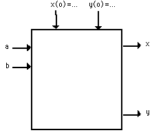
Figure 7. Blackbox PLANET model
Pascal notation (form 7)
These statements placed one after the other, look like this:
a:=1.0;
b:=0.5;
x;=0;
y:=0.5;
Repeat
... t := t + dt;
... dxdt := a;
... dydt := b;
... x := x + dxdt * dt;
... y := y + dydt * dt;
Until t > Tmax {=10.0}
7. An example: AORTA
As an example of the preceding paragraphs the various ways of representation of a simple model from the medical section are shown here. The model will be functionally described without really going into detail. For a description of the educational possibilities of this model the reader is referred to the description of the computer simulation program AORTA by Min (1982)
Introduction
In early phase of their studies medical students can familiarize themselves with some basic concepts from hemodynamics and some aspects of arteriosclerosis. In using this program an answer is given to questions like
'What happens if the total peripheral resistance of the circulation is increased?'
The opposite can also be an educational goal, namely the question as to what is the cause of the deviating picture of the diastolic pressure in the aorta.
'Can the cause of a decreased diastolic pressure in the aorta be a decreased compliance of the aorta? Yes or no?'
Students learn to handle notions like compliance and total peripheral resistance and changes there in. Students are supposed to be able to formulate questions and/or hypotheses and to verify these hypotheses with the help of this simulation program.
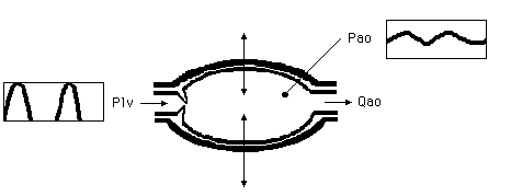
Figure 8. Conceptual model of a beating aorta. On the left blood is supplied
with a certain regularity and on the right blood is transported further into
the body. Changes in the pressure in the aorta of the human body are
indicated by Pao. Plv and Pao are variables.
Within the framework of a course about arteriosclerosis, case studies has been developed about the hardening of the wall of the aorta and the increased total resistance of the peripheral circulation. In this case study the students themselves have to recognize that the mean peripheral stream has changed and they have to try to restore it by adapting the pressure of the ventricle. The program is intended to teach the students how to deal with basal hemodynamic relations such as between pressure, compliance and volume and those between stream, resistance and pressure and to determine the consequences of interventions in hemodynamic variables.
Conceptual model (visual and textual)
The conceptual model of a beating aorta of a human being looks like the drawing in figure 8. The aorta is the great artery which springs from the left ventricle in the heart. The heart pumps (with a certain pressure, here Plv) a quantity of blood through the human body with each heart beat (Qao) attended by a change in pressure in the aorta. The aorta itself is elastic. The quantity which plays a role in the elasticity of the aorta is compliance (Cao). There is a connection between the form of the changes in pressure in the aorta and compliance. Furthermore there is a connection between the blood pressure in the aorta (Pao), the quantity of blood which flows through the aorta (Qao) and the resistance offered by the body (the peripheral resistance, Rp). The interesting variable to be measured externally, 'the pulse pressure', is practically equal to the pressure of the aorta. This pressure varies considerably and is very characteristic.
Block scheme
An inventory of this model, textual represented above, gives the following results:
- ventricle pressure Plv in mmHg (input variables)
- blood pressure in the aorta Pao in mmHg (output variables)
- blood volume Vao in ml (state variable)
- blood flow per time unit (flow) at the entrance of the aorta (Qao) (state variable)
- blood flow per time unit (flow) at the exit of the aorta (which is equal to the total blood
- flow through the body: the peripheral flow) (Qp) (state variable)
- maximum (left) ventricle pressure Plvmax in mmHg (model parameter)
- heart frequency f in 1/sec (model parameter)
- compliance of the aorta Cao (model parameter)
- peripheral resistance Rp (model parameter)
One can speak of one output variable, one input variable, three state variables and four (model)parameters which can serve as intervention possibilities. In figure 9 this is recapitulated in a block scheme. The model in the form of a system of integral equations.
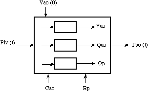
Figure 9. The block scheme of the pressure changes in the aorta. Plv(t) is the input
variable and Pao(t) the output variable. Cao,Rp, Vao(0) and Plv(t) can be used as intervention possibilities.
The pascal way of notation
The model of AORTA consist of four algebraic and one integral equation:
Plv = Plvmax . sin (2 . 3,14 . f . t) ( if Plv < 0 then Plv = 0 !)
Qao = 33 (Plv - Pao) ( if Plv < Pao then Qao = 0 !)
Qp = Pao / Rp
Tmax
Vao = ∫ (Qao - Qp) . dt + Vao(0)
0
Pao = Vao / Cao
NB. Op de plaats van het vraagteken hoort een integraal-teken te staan.
For the sake of convenience, the input variable is approached by half a sinus.
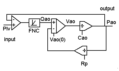
Figure 10. The analogue notation of the model of the pressure changes in the
aorta. The computer simulation program AORTA.
Analogue notation
Of this model a complete analogue scheme can be made as can be seen in figure 10. The non-linear function of conveyance is represented by a function block with the name FNC.
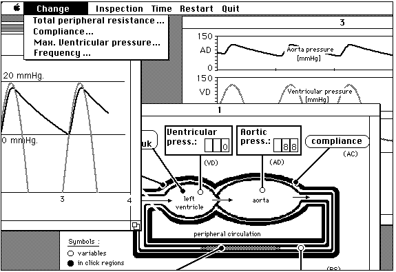
Figure 11. The complete computer simulation program AORTA. One window with the conceptual model and 'inclick regions' and two 'output windows' with different graphical presentations of the model variables.
At the input of the integrator the variable Qao - Qp (a difference of two flows) can be seen. This variable is one volume unit per second and is averaged 0. At the output of the integrator is the variable Vao (a volume with a volume unit). That lines up with what has been said before about an integrator, namely that at the input the variable differs only a factor time from the variable at the output. In this scheme it can be seen immediately that Cao, RP, but also Plv can be used as intervention possibilities. They are independent quantities. They appear not to depend on any other variable.
Pascal notation
The model in Pascal looks as follows, apart from details:
Repeat
t := t + dt;
Plv := Plvmax*sin(2 * 3.14 * f * t); if (Plv < 0.0) then Plv := 0.0;
Qao := 33 * (Plv - Pao); if (Plv < Pao) then Qao := 0.0;
Pao := Vao / Cao;
dVaodt := Qao - Pao / RP;
Vao := Vao + dVaodt * dt;
Until t > Tmax
The integration statements (here only one) are best all taken at the end, so that it is certain that the old and new values of the variables will not become mixed up.
Java notation
The model in Java looks as follows, apart from details:
public boolean stepModel()
{
t = t + dt;
PLV = PLVmax * Math.sin(2 * 3.14 * F * t);
if (PLV < 0.0) {PLV = 0.0;}
QAO = 33.0 * (PLV - PAO);
if ((PLV - PAO) < 0) {QAO = 0.0;}
VAO = VAO + (QAO - QP)*dt;
QP = PAO / RP;
PAO = VAO / CAO;
return t<Tmax;
}
Results (with AORTA)
In figure 11 the blood pressure can be seen at specific and characteristic values of peripheral resistance (Rp) and compliance (Cao). In one case built in the program it can be seen that the pressure during the systole has become high and in a second case the medical student can see that the pressure during the diastole is low. A first year medical student has to be able to diagnose in the first case of these 'clinical pictures' that something is wrong with the peripheral resistance and in the second case with the compliance. After that an experiment has to show if a change (upwards or downwards) of the peripheral resistance of compliance brings any improvement. If the 'patient' only becomes worse the students' hypothesis was wrong.